Download our e-book of Introduction To Python
Related Blog
Matplotlib - Subplot2grid() FunctionDiscuss Microsoft Cognitive ToolkitMatplotlib - Working with ImagesMatplotlib - PyLab moduleMatplotlib - Working With TextMatplotlib - Setting Ticks and Tick LabelsCNTK - Creating First Neural NetworkMatplotlib - MultiplotsMatplotlib - Quiver PlotPython - Chunks and Chinks View More
Top Discussion
How can I write Python code to change a date string from "mm/dd/yy hh: mm" format to "YYYY-MM-DD HH: mm" format? Which sorting technique is used by sort() and sorted() functions of python? How to use Enum in python? Can you please help me with this error? I was just selecting some random columns from the diabetes dataset of sklearn. Decision tree is a classification algo...How can it be applied to load diabetes dataset which has DV continuous Objects in Python are mutable or immutable? How can unclassified data in a dataset be effectively managed when utilizing a decision tree-based classification model in Python? How to leave/exit/deactivate a Python virtualenvironment Join Discussion
Top Courses
Webinars
Project 4: Prediction of salary Based on years of experience

Shashank Shanu
2 years ago

Table of Contents
- Problem Statement
- Dataset description
- Model Building
- Visualization
- Model Evaluation
- Conclusion
Problem Statement
To build a machine learning model and predict the salary of the employees based on year of experience
Dataset description
- This dataset is randomly created to show you how we can use machine learning technique and build a Linear Regression model to predict the salary of an employee based on years of experience.
- This dataset consists of two columns
- Salary- Represent the salary of a person.
- Years- Years of experience
- Note: - It's a small dataset which is being used for only demo purpose.
Importing libraries
import pandas as pd
import numpy as np
Importing data
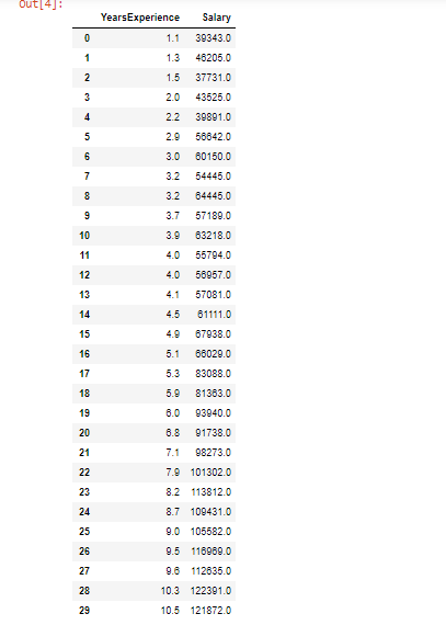
data = pd.read_csv("Salary_Dataa.csv")Displaying dataset
dataOutput:
Checking shape of dataset
data.shapeOutput:
(30, 2)- We can see that our dataset consists of 30 observations and 2 rows only. These are very small dataset as it is created randomly to show how we can build a regression model.
Checking dataset information
data.info()Output:
RangeIndex: 30 entries, 0 to 29
Data columns (total 2 columns):
 #   Column           Non-Null Count  Dtype
---  ------           --------------  -----
 0   YearsExperience  30 non-none     float64
 1   Salary           30 non-none     float64
dtypes: float64(2)
memory usage: 608.0 bytes- We can see that both the variables are of float data types
Checking for none values
data.isnone().count()Output:
YearsExperience    30
Salary             30
dtype: int64- We can see that there are no missing values are present in our dataset
Model Building
Splitting of dataset into independent and dependent variables
X = data.iloc[:,:-1].values
Y = data.iloc[:,1].values
Independent variable
XOutput:
array([[ 1.1],
       [ 1.3],
       [ 1.5],
       [ 2. ],
       [ 2.2],
       [ 2.9],
       [ 3. ],
       [ 3.2],
       [ 3.2],
       [ 3.7],
       [ 3.9],
       [ 4. ],
       [ 4. ],
       [ 4.1],
       [ 4.5],
       [ 4.9],
       [ 5.1],
       [ 5.3],
       [ 5.9],
       [ 6. ],
       [ 6.8],
       [ 7.1],
       [ 7.9],
       [ 8.2],
       [ 8.7],
       [ 9. ],
       [ 9.5],
       [ 9.6],
       [10.3],
       [10.5]])
Dependent variable
YOutput:
array([ 39343.,  46205.,  37731.,  43525.,  39891.,  56642.,  60150.,
        54445.,  64445.,  57189.,  63218.,  55794.,  56957.,  57081.,
        61111.,  67938.,  66029.,  83088.,  81363.,  93940.,  91738.,
        98273., 101302., 113812., 109431., 105582., 116969., 112635.,
       122391., 121872.])
Plotting Scatter plot to check relationship between independent variable and dependent variable
import matplotlib.pyplot as plt

plt.scatter(X,Y,color = "blue")
Output:
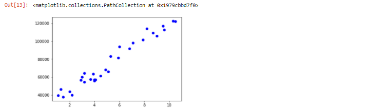
- We can observe that the independent and dependent variable is linearly related to each other
Splitting dataset for training set and testing set
from sklearn.model_selection import train_test_split

x_train,x_test,y_train,y_test = train_test_split(X,Y,test_size=0.33,random_state = 0)
Displaying x_train
x_trainOutput:
array([[ 2.9],
       [ 5.1],
       [ 3.2],
       [ 4.5],
       [ 8.2],
       [ 6.8],
       [ 1.3],
       [10.5],
       [ 3. ],
       [ 2.2],
       [ 5.9],
       [ 6. ],
       [ 3.7],
       [ 3.2],
       [ 9. ],
       [ 2. ],
       [ 1.1],
       [ 7.1],
       [ 4.9],
       [ 4. ]])
Displaying y_train
y_trainOutput:
array([ 56642.,  66029.,  64445.,  61111., 113812.,  91738.,  46205.,
       121872.,  60150.,  39891.,  81363.,  93940.,  57189.,  54445.,
       105582.,  43525.,  39343.,  98273.,  67938.,  56957.])
Displaying y_test
y_testOutput:
array([ 37731., 122391.,  57081.,  63218., 116969., 109431., 112635.,
        55794.,  83088., 101302.])
Fitting Simple Linear regression to the training set
from sklearn.linear_model import LinearRegression
regressor = LinearRegression()
regressor.fit(x_train,y_train)
Output:
LinearRegression(copy_X=true, fit_intercept=true, n_jobs=none, normalize=false)Predicting the Test set results
y_pred = regressor.predict(x_test)Displaying y_pred (Predicted salary)
y_pred Output:
array([ 40835.10590871, 123079.39940819,  65134.55626083,  63265.36777221,
       115602.64545369, 108125.8914992 , 116537.23969801,  64199.96201652,
        76349.68719258, 100649.1375447 ])
Displaying y_test (Real salary)
y_test Output:
array([ 37731., 122391.,  57081.,  63218., 116969., 109431., 112635.,
        55794.,  83088., 101302.])
Calculating Error/ Residue
residue = y_pred - y_test    # residue or error between actual and predicted salary
residue
Output:
array([ 3104.10590871,   688.39940819,  8053.55626083,    47.36777221,
       -1366.35454631, -1305.1085008 ,  3902.23969801,  8405.96201652,
       -6738.31280742,  -652.8624553 ])
Visualization
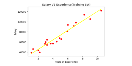
Visualizing the training set results
plt.scatter(x_train,y_train,color="red")
plt.plot(x_train,regressor.predict(x_train),color="yellow")
plt.title("Salary VS Experience(Training Set)")
plt.xlabel("Years of Experience")
plt.ylabel("Salary")
plt.show()
Output:
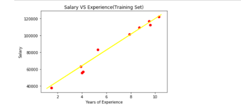
Visualizing the testing set results
plt.scatter(x_test,y_test,color="Red")
plt.plot(x_train,regressor.predict(x_train),color="yellow")
plt.title("Salary VS Experience(Training Set)")
plt.xlabel("Years of Experience")
plt.ylabel("Salary")
plt.show()
Output:
Calculating Intercept and Coefficient
print(regressor.coef_)
print(regressor.intercept_)
Output:
[9345.94244312]
26816.192244031176y_test.shapeOutput:
(10,)y_pred.shapeOutput:
(10,)Model Evaluation
from sklearn.metrics import r2_score
from sklearn.metrics import mean_squared_error

rmse = np.sqrt(mean_squared_error(y_test,y_pred))
r2 = r2_score(y_test,y_pred)                           #built-in function r2_score() indicates R-squared value

print("RMSE =", rmse)
print("R2 Score=",r2)
Output:
RMSE = 4585.415720467589
R2 Score= 0.9749154407708353
Conclusion
- In this small project, We saw how we can build a machine learning model ie., Regression model and predict the salary of the employees based on years of experience.
- Here, We build a regression model and check the model RMSE which is equal to 4585.415720467589.
- We also checked for R2 score of our model which is equal to 0.9749154407708353 or 97%. Which is a very good R2 score.
I hope you enjoyed this project and also you came to know about how we can use and implement Linear Regression Algorithm.
For more such blogs/courses on data science, machine learning, artificial intelligence and emerging new technologies do visit us at https://insideaiml.com/home.
Thanks for reading…
Happy Learning…