Download our e-book of Introduction To Python
Related Blog
Matplotlib - Subplot2grid() FunctionDiscuss Microsoft Cognitive ToolkitMatplotlib - Working with ImagesMatplotlib - PyLab moduleMatplotlib - Working With TextMatplotlib - Setting Ticks and Tick LabelsCNTK - Creating First Neural NetworkMatplotlib - MultiplotsMatplotlib - Quiver PlotPython - Chunks and Chinks View More
Top Discussion
How can I write Python code to change a date string from "mm/dd/yy hh: mm" format to "YYYY-MM-DD HH: mm" format? Which sorting technique is used by sort() and sorted() functions of python? How to use Enum in python? Can you please help me with this error? I was just selecting some random columns from the diabetes dataset of sklearn. Decision tree is a classification algo...How can it be applied to load diabetes dataset which has DV continuous Objects in Python are mutable or immutable? How can unclassified data in a dataset be effectively managed when utilizing a decision tree-based classification model in Python? How to leave/exit/deactivate a Python virtualenvironment Join Discussion
Top Courses
Webinars
How to Explain Machine Learning Model in Interview?

Nuthan Nittya
2 years ago

Table of Contents
- Introduction
- Models Covered
1. Linear Regression
2. Ridge Regression
3. Lasso Regression
4. Logistic Regression
5. K Nearest-Neighbours
6. Naive Bayes
7. Support Vector Machines
8. Decision Trees
9. Random Forests
10. AdaBoost
11. Gradient Boost
12. XGBoost
Introduction
In preparation for any interviews, I wanted to share a resource that provides concise explanations of the machine learning model. They are not meant to be extensive, rather the opposite. Hopefully, by reading this, you’ll have a sense of how you can communicate complex models in a simple manner.
Models Covered
- Linear Regression
- Ridge Regression
- Lasso Regression
- Logistic Regression
- K Nearest-Neighbours
- Naive Bayes
- Support Vector Machines
- Decision Trees
- Random Forests
- AdaBoost
- Gradient Boost
- XGBoost
1. Linear Regression
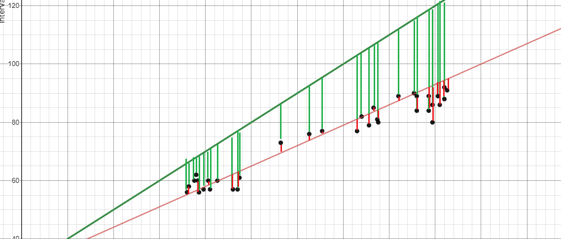
Linear Regression involves finding a ‘line of best fit’ that represents a dataset using the least-squares method. The least-squares method involves finding a linear equation that minimizes the sum of squared residuals. A residual is equal to the actual minus predicted value.
To give an example, the red line is a better line of best fit than the green line because it is closer to the points, and thus, the residuals are smaller
2. Ridge Regression
Ridge regression, also known as L1 Regularization, is a regression technique that introduces a small amount of bias to reduce overfitting. It does this by minimizing the sum of squared residuals plus a penalty, where the penalty is equal to lambda times the slope squared. Lambda refers to the severity of the penalty.
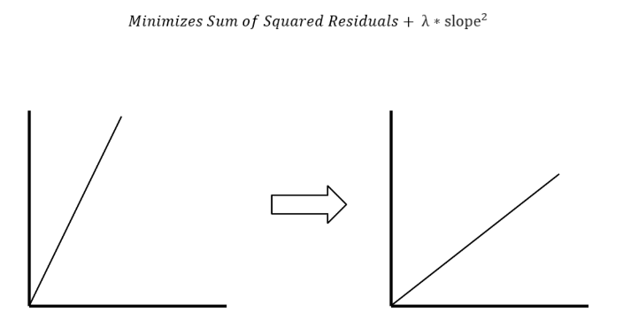
Without a penalty, the line of best fit has a steeper slope, which means that it is more sensitive to small changes in X. By introducing a penalty, the line of best fit becomes less sensitive to small changes in X. This is the idea behind ridge regression.
3. Lasso Regression
Lasso Regression, also known as L2 Regularization, is similar to Ridge regression. The only difference is that the penalty is calculated with the absolute value of the slope instead.

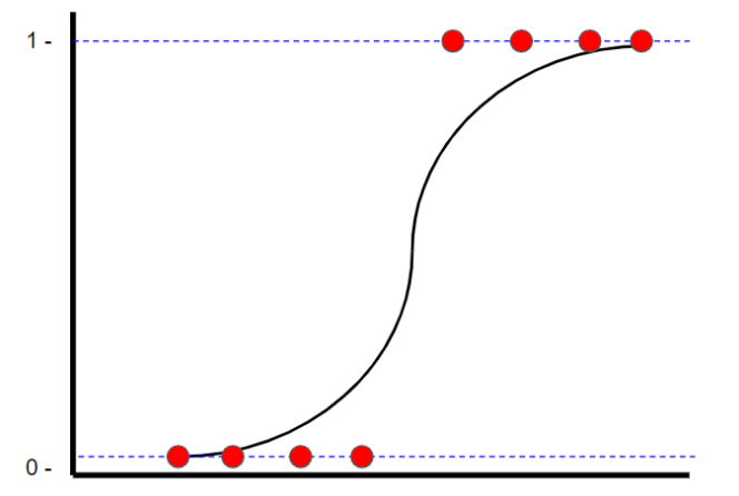
4. Logistic Regression
Logistic Regression is a classification technique that also finds a ‘line of best fit’. However, unlike linear regression where the line of best fit is found using least squares, logistic regression finds the line (logistic curve) of best fit using maximum likelihood. This is done because the y value can only be one or zero.
5. K-Nearest Neighbours
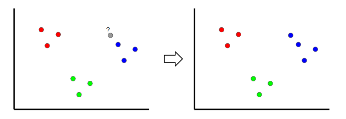
K-Nearest Neighbours is a classification technique where a new sample is classified by looking at the nearest classified points, hence ‘K-nearest’. In the example above, if k=1 then an unclassified point would be classified as a blue point.
If the value of k is too low, it can be subject to outliers. However, if it’s too high, it may overlook classes with only a few samples.
6. Naive Bayes
The Naive Bayes Classifier is a classification technique inspired by Bayes Theorem, which states the following equation:
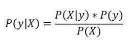
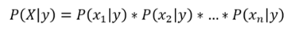
Also, since we are solving for y, P(X) is a constant which means that we can remove it from the equation and introduce a proportionality.
Thus, the probability of each value of y is calculated as the product of the conditional probability of xn given y.
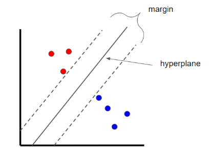
7. Support Vector Machines
Support Vector Machines are a classification technique that finds an optimal boundary, called the hyperplane, which is used to separate different classes. The hyperplane is found by maximizing the margin between the classes.
8. Decision Trees
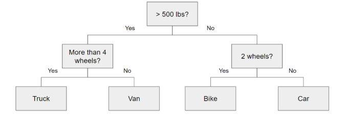
A decision tree is essentially a series of conditional statements that determine what path a sample takes until it reaches the bottom. They are intuitive and easy to build but tend not to be accurate.
9. Random Forest
Random Forest is an ensemble technique, meaning that it combines several models into one to improve its predictive power. Specifically, it builds 1000s of smaller decision trees using bootstrapped datasets and random subsets of variables (also known as bagging). With 1000s of smaller decision trees, Random forests use a ‘majority wins’ model to determine the value of the target variable.
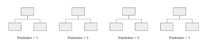
For example, if we created one decision tree, the third one, it would predict 0. But if we relied on the mode of all 4 decision trees, the predicted value would be 1. This is the power of random forests.
10. AdaBoost
AdaBoost is a boosted algorithm that is similar to Random Forests but has a couple of significant differences:
- Rather than a forest of trees, AdaBoost typically makes a forest of stumps (a stump is a tree with only one node and two leaves).
- Each stump’s decision is not weighted equally in the final decision. Stumps with less total error (high accuracy) will have a higher say.
- The order in which the stumps are created is important, as each subsequent stump emphasizes the importance of the samples that were incorrectly classified in the previous stump.
11. Gradient Boost
Gradient Boost is similar to AdaBoost in the sense that it builds multiple trees where each tree is built off of the previous tree. Unlike AdaBoost which builds stumps, Gradient Boost builds trees with usually 8 to 32 leaves.
More importantly, Gradient differs from AdaBoost in the way that the decisions trees are built. Gradient boost starts with an initial prediction, usually the average. Then, a decision tree is built based on the residuals of the samples. A new prediction is made by taking the initial prediction + a learning rate times the outcome of the residual tree, and the process is repeated.
12. XGBoost
XGBoost is essentially the same thing as Gradient Boost, but the main difference is how the residual trees are built. With XGBoost, the residual trees are built by calculating similarity scores between leaves and the preceding nodes to determine which variables are used as the roots and the nodes.
Liked what you read? Then don’t break the spree. Visit our insideAIML blog page to read more awesome articles.
Or if you are into videos, then we have an amazing Youtube channel as well. Visit our InsideAIML Youtube Page to learn all about Artificial Intelligence, Deep Learning, Data Science and Machine Learning.
Keep Learning. Keep Growing.