How To Train Neural Network?

                 Gradient Descent Optimization Technique

                 1. Dropout

                 2. Early Stopping

                 3. Data Augmentation

                 4. Transfer Learning

          As we know, one of the most important parts of deep learning is training the neural networks. So, let's learn how it actually works. In this article, we will try to learn how a neural network gets to train. We will also learn about the feed-forward method and backpropagation method in Deep Learning.

          Training in deep learning is the process that helps machines to learn about the function/equation. We have to find the optimal values of the weights of a neural network to get the desired output.

To train a neural network, we use the iterative method using gradient descent. Initially, we start with random initialization of the weights. After random initialization of the weights, we make predictions on the data with the help of forward-propagation method, then we compute the corresponding cost function C, or loss and update each weight w by an amount proportional to dC/dw, i.e., the derivative of the cost functions w.r.t. the weight. The proportionality constant is known as the learning rate.

Now, you might be thinking what is learning rate?

The learning rate is a type of hyper-parameter that helps us to controls the weights of our neural network with respect to the loss gradient. It gives us an idea of how quickly the neural network updates the concepts it has learned.

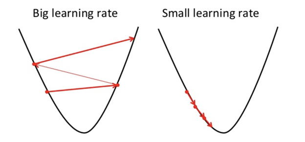
A learning rate should not be too low as it will take more time to converge the network and it should also not be even too high as the network may never converge. So, it is always desirable to have an optimal value of learning rate so that the network converges to something useful.

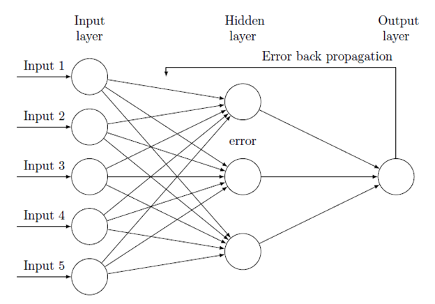
We can calculate the gradients efficiently using the back-propagation algorithm. The key observation of backward propagation or backward prop is that because of the chain rule of differentiation, the gradient at each neuron in the neural network can be calculated using the gradient at the neurons, it has outgoing edges too. Hence, we calculate the gradients backwards, i.e., first calculate the gradients of the output layer, then the top-most hidden layer, followed by the preceding hidden layer, and so on, ending at the input layer.

The back-propagation algorithm is implemented mostly using the idea of a computational graph, where each neuron is expanded into many nodes in the computational graph and performs a simple mathematical an operation like addition, multiplication.

The computational graph does not have any weights on the edges; all weights are assigned to the nodes, so the weights become their own nodes. The backward propagation algorithm is then run on the computational graph. Once the calculation is complete, only the gradients of the weight nodes are required for the update. The rest of the gradients can be discarded.

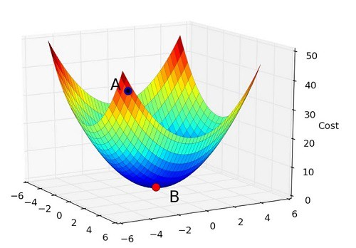
          The gradient is nothing but it is the slope, and slope, on an x-y graph, represents how two variables are related to each other: the rise over the run, the change in distance over the change in time, etc. In this case, the slope is the ratio between the network’s error and a single weight; i.e., how does the error change as the weight is varied.

To put it in a straight forward way, here we mainly want to find which weights which produces the least error. We want to find the weights that correctly represents the signals contained in the input data, and translates them to correct classification.

As a neural network learns, it slowly adjusts many weights so that they can map signal to meaning correctly. The ratio between network Error and each of those weights is a derivative, dE/dw that calculates the extent to which a slight change in weight causes a slight change in the error.

Each weight is just one factor in a deep neural a network that involves many transforms; the signal of the weight passes through activations functions and then sums over several layers, so we use the chain rule of calculus to work back through the network activations and outputs. This leads us to the weight in question, and its relationship to the overall error.

Given two variables, error and weight, are mediated by a third variable, activation, through which the weight is passed. We can calculate how a change in weight affects a change in error by first calculating how a change in activation affects a change in Error, and how a change in weight affects a change in activation.

The basic idea in deep learning is nothing more than that adjusting a model’s weights in response to the error it produces, until you cannot reduce the error any more.

The deep net trains slowly if the gradient value is small and fast if the value is high. Any inaccuracies in training lead to inaccurate outputs. The process of training the nets from the output back to the input is called backpropagation or back prop. We know that forward propagation starts with the input and works forward. Back prop does the reverse/opposite calculating the gradient from right to left.

Each time we calculate a gradient, we use all the previous gradients up to that point.

Let us start at a node in the output layer. The edge uses the gradient at that node. As we go back into the hidden layers, it gets more complex. The product of two numbers between 0 and 1 gives you a smaller number. The gradient value keeps getting smaller and as a result, back prop takes a lot of time to train and produces bad accuracy.

          There are certain challenges for both shallow neural networks and deep neural networks, like overfitting and computation time.

DNNs are easily affected by overfitting because the use of added layers of abstraction which allow them to model rare dependencies in the training data.

Regularization methods such as drop out, early stopping, data augmentation, and transfer learning are used during training to combat the problem of overfitting.

Drop out regularization randomly omits units from the hidden layers during training which helps in avoiding rare dependencies. DNNs take into consideration several training parameters such as the size, i.e., the number of layers and the number of units per layer, the learning rate and initial weights. Finding optimal parameters is not always practical due to the high cost in time and computational resources. Several hacks such as batching can speed up computation. The large processing power of GPUs has significantly helped the training process, as the matrix and vector computations required are well-executed on the GPUs.

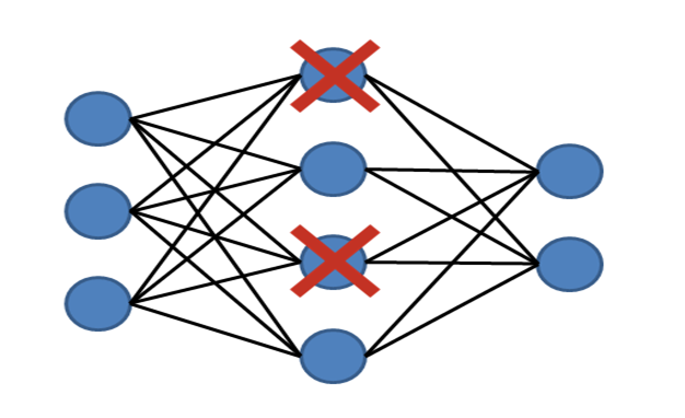
          Dropout is a well-known regularization technique for neural networks. Deep neural networks are particularly prone to overfitting.

Let us now see what dropout is and how it works.

In the words of Geoffrey Hinton, one of the pioneers of Deep Learning, ‘If you have a deep neural net and it's not overfitting, you should probably be using a bigger one and using dropout’.

Dropout is a technique where during each iteration of gradient descent, we drop a set of randomly selected nodes. This means that we ignore some nodes randomly as if they do not exist.

Each neuron is kept with a probability of q and dropped randomly with probability 1-q. The value q may be different for each layer in the neural network. A value of 0.5 for the hidden layers, and 0 for input layer works well on a wide range of tasks.

During evaluation and prediction, no dropout is used. The output of each neuron is multiplied by q so that the input to the next layer has the same expected value.

The idea behind Dropout is as follows − In a neural network without dropout regularization, neurons develop co-dependency amongst each other, that leads to overfitting.

Implementation trick :- Dropout is implemented in libraries such as TensorFlow and Pytorch by keeping the output of the randomly selected neurons as 0. That is, though the neuron exists, its output is overwritten as 0.

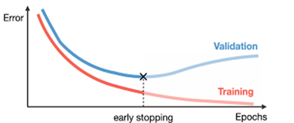
          Here we try to train neural networks using an iterative an algorithm called gradient descent.

The idea behind early stopping is intuitive; we stop training when the error starts to increase. Here, by error, we mean the error measured on validation data, which is the part of training data used for tuning hyper-parameters. In this case, the hyper-parameter is the stop criteria.

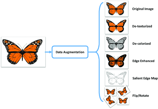
          It is a process where we increase the quantum of data we have or augment it by using existing data and applying some transformations on it. The exact transformations used to depend on the task we intend to achieve. Moreover, the transformations that help the neural net depend on its architecture.

For instance, in many computer vision tasks such as object classification, an effective data augmentation technique is adding new data points that are cropped or translated versions of original data.

When a computer accepts an image as an input, it takes in an array of pixel values. Let us say that the whole image is shifted left by 15 pixels. We apply many different shifts in different directions, resulting in an augmented dataset many times the size of the original dataset.

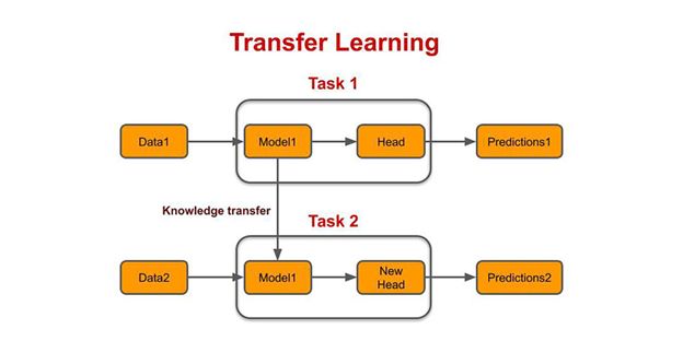
          The process of taking a pre-trained model and “fine-tuning” the model with our own dataset is called transfer learning. There are several ways to do this. A few ways are described below −

The concept behind this is that the pre-trained model will act as a feature extractor, and only the last layer will be trained on the current task.

I hope you liked this article.

 

Enjoyed reading this blog? Then why not share it with others. Help us make this AI community stronger. 

To learn more about such concepts related to Artificial Intelligence, visit our insideAIML blog page.

You can also ask direct queries related to Artificial Intelligence, Deep Learning, Data Science and Machine Learning on our live insideAIML discussion forum.

Keep Learning. Keep Growing.